The butterfly effect is the popular concept that “the flap of a butterfly’s wings in Brazil can set off a tornado in Texas”. This idea, which is in fact misunderstood and misrepresented in many occasions, came from the seminal work of Edward Lorenz, which was conducting methereological simulations. In this brief post, I will reproduce its experiment using a basic numpy simulation to show the origin of its incredible discovery.

The Lorenz system

In 1963, Edward Lorenz developed a simplified mathematical model for atmospheric convection. The model is a system of three ordinary differential equations which are now named after him:

this sets of equation can not be solved analytically but Lorenz had an early electronic computer, called the Royal McBee, whose vacuum tubes could perform sixty ($60$!) multiplications a second. This seems ridicolous when compared to modern-day computers, but it is still way faster than a human. In fact Lorenz did not conduct this set of equations, but with a more complex one using $12$ variables. This model was later devoloped by him to see whether even such a(n apparently) simple system displayed the puzzling phenomenon.

The experiment

We will now try to reproduce a modern version of his experiment, using the $3$-variable model, as it is simpler (and nicer to plot). After the usual imports

import numpy as np
import matplotlib.animation as animation
import matplotlib.pyplot as plt
import time
np.set_printoptions(precision=3)

%matplotlib inline

we can easily write our system equations:

def Lorenz(V, sigma, b, r):
    x, y, z = V
    
    x_dot = -sigma*x+ sigma*y
    y_dot = -x*z + r*x - y
    z_dot = x*y - b*z
    
    dV = np.array([x_dot,y_dot,z_dot])
    return dV 

Let us use the set of parameters for which the phenomenon is evident, setting $\sigma = 10$, $\beta = 8/3$ and $\rho = 28$.

s = 10 #sigma
b = 8./3 #beta
r = 28 #rho

We then decide to let the system evolve for $T = 100000$ steps, each one of length $dt =0.001$s.

T = 100000
dt = 0.001

We also set the initial condition to $(x,y,z)=(1,1,1)$:

S = np.zeros([T+1,3]) #array to be filled
S[0] = np.array( [1., 1., 1.] ) #initial condition

Now we are ready to run the simulation. We will use the Euler method to integrate the set of equation: I know it is really bad, but we are not interested in a proper integration, we are just trying to prove a point.

#print the initial condition
print (0, S[0]) 

for i in range(0, T):
    S[i+1] = S[i] + Lorenz(S[i], s, b, r)*dt #numerical integration using Euler method
    #we only print 1 value every 1000
    if ((i+1)%1000 == 0):
        print (i+1, S[i+1])

The output will be:

0 [1. 1. 1.]
1000 [-9.109 -8.42  28.648]
2000 [-8.333 -9.375 25.358]
3000 [-7.648 -6.722 27.223]
4000 [ -9.852 -10.292  28.164]
5000 [-6.927 -7.55  24.184]
6000 [-9.198 -7.206 30.215]
7000 [ -8.323 -10.533  23.516]
8000 [-6.462 -4.633 27.122]
9000 [-10.824 -13.256  26.888]
10000 [-4.398 -3.841 23.225]
11000 [-12.279 -15.658  27.846]
12000 [-2.521 -0.09  24.718]
13000 [ 2.99   4.914 15.325]
14000 [-1.015 -1.972  7.059]
15000 [11.014  8.951 32.458]
16000 [ 5.374  7.141 19.872]
17000 [10.779  5.93  34.767]
18000 [ 2.207  2.876 17.304]
19000 [-2.262 -4.254  8.872]
20000 [10.611  5.877 34.481]
21000 [ 2.632  3.579 17.188]
22000 [2.411 4.574 8.422]
23000 [-9.889 -5.085 33.742]
24000 [-3.319 -4.794 16.82 ]
25000 [ -9.802 -16.873  16.542]
26000 [ 4.467 -0.578 29.194]
27000 [-2.344 -4.267 21.145]
28000 [-11.51  -17.193  23.029]
29000 [-14.802  -6.776  42.19 ]
30000 [ 2.714  3.523 17.851]
31000 [ 4.892  9.069 10.291]
32000 [-7.814 -1.713 32.816]
33000 [ 0.098  0.509 16.533]
34000 [-6.556 -9.648 19.628]
35000 [-7.847 -2.61  32.07 ]
36000 [-2.407 -3.65  15.303]
37000 [ 7.257 13.131 12.609]
38000 [-5.922 -0.244 30.85 ]
39000 [ 1.571  2.781 17.712]
40000 [-3.534 -6.532  9.998]
41000 [10.062  3.851 35.13 ]
42000 [ 0.217 -0.281 17.976]
43000 [ 3.908  6.527 24.046]
44000 [11.475  9.958 32.464]
45000 [ 4.733  6.073 19.84 ]
46000 [12.599  9.271 35.631]
47000 [ 1.229  0.734 19.629]
48000 [-5.628 -9.316 15.314]
49000 [-14.652 -21.099  27.784]
50000 [ 2.349  0.977 22.797]
51000 [-1.682 -2.972 11.913]
52000 [13.725 14.364 33.318]
53000 [ 1.384 -1.338 24.537]
54000 [ 3.558  5.561 18.051]
55000 [14.32  17.302 31.618]
56000 [-12.871 -22.525  18.731]
57000 [ 4.995  5.092 22.731]
58000 [12.354 11.597 32.839]
59000 [ 3.124  3.444 19.94 ]
60000 [ 9.888 16.199 18.481]
61000 [-14.574  -6.886  41.651]
62000 [ 1.903  2.197 18.079]
63000 [-3.731 -6.831 10.479]
64000 [10.631  4.139 35.972]
65000 [-0.378 -1.549 19.888]
66000 [ 5.242  8.857 14.377]
67000 [-1.352 -2.695  5.728]
68000 [ 9.765  6.936 31.744]
69000 [ 6.932  9.514 20.66 ]
70000 [ 7.387  3.21  30.627]
71000 [ 5.607  8.731 16.768]
72000 [13.441  7.706 38.72 ]
73000 [-7.756  3.758 36.869]
74000 [ 6.069  9.178 17.828]
75000 [10.391  3.494 36.031]
76000 [-0.707 -2.39  21.298]
77000 [ 1.19   2.16  10.609]
78000 [-12.837 -12.699  32.87 ]
79000 [-2.257 -1.808 20.748]
80000 [ 0.085  0.167 10.009]
81000 [-7.353 -9.682 22.917]
82000 [-7.199 -4.701 28.652]
83000 [ -9.785 -12.898  24.285]
84000 [-4.711 -3.169 25.085]
85000 [-10.384 -15.104  22.603]
86000 [-4.251  0.481 28.723]
87000 [ 2.463  4.162 19.653]
88000 [10.584 17.009 19.786]
89000 [-13.82   -5.01   41.453]
90000 [ 1.99   2.446 17.652]
91000 [-3.627 -6.695 10.079]
92000 [10.035  3.739 35.17 ]
93000 [ 0.077 -0.521 18.164]
94000 [ 5.557  8.167 19.575]
95000 [ 9.75   4.346 34.116]
96000 [ 2.053  2.814 16.549]
97000 [-5.468 -9.997 11.202]
98000 [ 8.145  1.338 33.719]
99000 [-1.164 -2.479 19.464]
100000 [ 2.126  3.898 10.076]

So, we started from [1,1,1] and after $100000$ steps we are at [ 2.126 3.898 10.076]. Let us plot the trajectory to have an idea of what’s happening:

fig = plt.figure(figsize=(20,20))
ax = fig.gca(projection='3d')

ax.plot(S[:,0], S[:,1], S[:,2], 'b',lw=0.5)
ax.set_xlabel("X Axis")
ax.set_ylabel("Y Axis")
ax.set_zlabel("Z Axis")
ax.set_title("Lorenz Attractor")
plt.show()

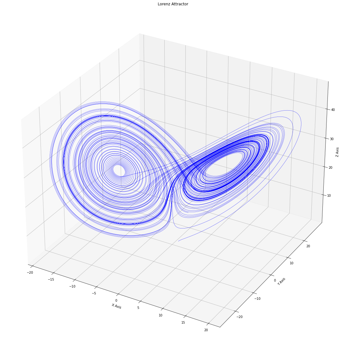
Lorenz wanted to examine some of the solutions in more detail, but calculation back in those days were terribly slow. He used the computer in his office, and he typed in some of the intermediate conditions which the computer had printed out as new initial conditions to start another computation. Let’s do the same.

As an intermediate condition, we will use $L = 7000$. So that out new simulation will start from S[L] = S[7000] = [ 7.387, 3.21, 30.627].

L = 70000 
# the values are: [ 7.387  3.21  30.627]
#so we create a new vector 
S_n = np.zeros([T+1,3])
#and we inizialize the 70000-th with those values
S_n[L] = np.array( [7.387,  3.210,  30.627] )

Now we can run our second simulation:

print (L, S_n[L])
for i in range(L, T): #this times the loop starts from L = 70000
    S_n[i+1] = S_n[i] + Lorenz(S_n[i], s, b, r)*dt
    if ((i+1)%1000 == 0):
        print (i+1, S_n[i+1])

and get

70000 [ 7.387  3.21  30.627]
71000 [ 5.606  8.729 16.767]
72000 [13.446  7.717 38.722]
73000 [-7.699  3.783 36.801]
74000 [ 6.066  9.181 17.81 ]
75000 [10.423  3.515 36.075]
76000 [-0.708 -2.441 21.446]
77000 [ 0.837  1.526 10.527]
78000 [-12.32  -13.557  30.625]
79000 [-3.018 -2.641 21.428]
80000 [ -6.874 -11.925  14.104]
81000 [14.219  7.514 40.47 ]
82000 [-0.418  0.552 20.113]
83000 [-4.377 -6.519 21.167]
84000 [-11.809  -8.484  34.632]
85000 [-2.687 -3.323 18.366]
86000 [-5.181 -9.522 10.804]
87000 [ 8.063  1.525 33.418]
88000 [-0.814 -1.765 18.077]
89000 [ 6.606 11.243 14.757]
90000 [-11.246 -19.779  16.915]
91000 [ 3.807  2.575 23.793]
92000 [ 8.281 13.504 17.31 ]
93000 [16.548 17.212 37.631]
94000 [-2.321 -2.179 20.054]
95000 [-1.017 -1.868  9.574]
96000 [12.314 11.754 32.596]
97000 [ 3.224  3.553 20.057]
98000 [10.657 16.915 20.273]
99000 [-16.88  -19.464  36.285]
100000 [ 3.401  3.836 20.04 ]

The final point for iteration number 100000 was [ 2.126 3.898 10.076], but now we are in a completly different point! How is this possible?
The whole process is deterministic, there is no place here for noise or stochasticity of any sort.

Let us plot both trajecories. This time I will highlight with a star the state at the 7000-tt step (the “starting” state) and with a dot the state they reached at the final iteration:

fig = plt.figure(figsize=(20,20))
ax = fig.gca(projection='3d')

ax.plot(S[L:,0], S[L:,1], S[L:,2], 'b', lw=0.8)

ax.plot(S_n[L:,0], S_n[L:,1], S_n[L:,2], 'r', lw=0.8)

ax.plot(S[L,0], S[L,1], S[L,2], 'b*', ms = 20)
ax.plot(S_n[L,0], S_n[L,1], S_n[L,2],  'r*', ms = 20)


ax.plot(S[-1,0], S[-1,1], S[-1,2], 'b.', ms = 20)
ax.plot(S_n[-1,0], S_n[-1,1], S_n[-1,2], 'r.', ms = 20)


ax.set_xlabel("X Axis")
ax.set_ylabel("Y Axis")
ax.set_zlabel("Z Axis")
ax.set_title("Lorenz Attractor")

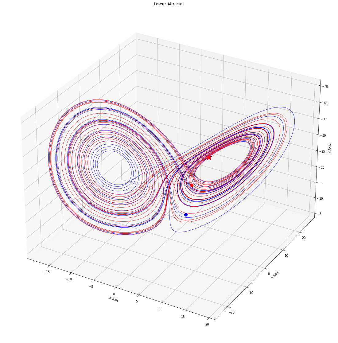
Apparently, the two systems start from the same point but, after a while, they diverge. To better see what’s happening, we also plot the distance between the two trajectories:

dist = []

for i in range(L,T):
    d = np.linalg.norm(S[i] - S_n[i])
    dist.append(d)
    
plt.plot(range(L,T), dist)
plt.title('Distance from the original trajectory')
plt.xlabel('timestep')
plt.ylabel('distance')
plt.show()

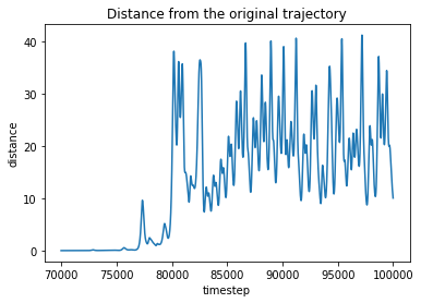
At first the two systems seem to stay quite close to each other, but aftwer a while their distance increases ad they end up having to really different orbits.
How is this possible?

Sensitive dependence on initial conditions

What we did was manually inserting the values into the initial state for the new simulation. This is what Lorenz did: he read some numbers and typed them back. The issue is (and was, for Lorenz) that the computer is printing numbers with a different precision than the one it is using for computation. For the the Lorenz case, the computer was using six decimal places, while he only typed in three (as we did). But the characteristic of the system he was studying were such that evena tiny difference due to a rounding error lead to macroscopic variation in the system state.

Lorenz narrated the story behind his discovery in an interview:

In the course of doing this I wanted to examine some of the solutions in more detail. I had a small computer in my office then so I typed in some of the intermediate conditions which the computer had printed out as new initial conditions to start another computation and then went out for awhile. When I came back I found that the solution was not the same as the one I had before. The computer was behaving differently. I suspected computer trouble at first. But I soon found that the reason was that the numbers I had typed in were not the same as the original ones. These were rounded off numbers. And the small difference between something retained to six decimal places and rounded off to three had amplified in the course of two months of simulated weather until the difference was as big as the signal itself. And to me this implied that if the real atmosphere behaved in this method then we simply couldn’t make forecasts two months ahead. The small errors in observation would amplify until they became large.

Scientists now refer to this phenomenon as sensitive dependence on initial conditions: systems which display this features ampliflies small differences in their starting points while evolving, ending up in different states as time passes. This fact has a crucial implication: let’s say that we are interested in predicting the system state in the future while kwowing the current state. This is the typical case in weather forecasting, for example. So, we go out and measure our system initial state $x(0)$. Then, we run our model to predict the future state for time $T$, $x(T)$. But for sure, our measuring of the initial state was not perfect: error are impossible to avoid when measuring something and our system was actually in the state $x_{\text{true}}(0)$. Of course, using better instruments it is possible to reduce the discrepancy between $x(0)$ and $x_{\text{true}}(0)$, but it will always be non-null.
Is this a proble? Well, it might. If our system displays sensitive dependence on initial conditions, this means that the small error we made will amplify as time passes and $x_{\text{true}}(T)$ will be totally different from $x_{\text{true}}(T)$. And it is important to remark that this happens even if your model is perfect! This is why weater forecasting is so difficult in practice: small errors amplify!

I hope that this brief introduction managed to make you excited as I am about this strange phenomena. Incoming posts are going to be devoted to deepen this fascinating topic.