This post is the English translation of an online article I published during the COVID-19 pandemic on Immoderati.it. At the time, I wanted to explain—using simple mathematical tools—how epidemiological models describe the spread of infectious diseases.

The central concept is a single number, $R_0$, which determines whether a disease will spread or die out. Every pathogen has its own $R_0$; for the coronavirus, early estimates placed it around 2.5.
If this number is less than 1, the disease will not spread; if it is greater than 1, an outbreak will occur, leading to the spread of the epidemic. But where does this number come from? What does it depend on? What does it really mean to say that it represents “the average number of people each infected person infects”? And how should we interpret it?

Since 2.5 is clearly not a very small value—so much so that we all found ourselves confined at home—I decided to write an article explaining the mathematics of contagion.

The SIR Model

This simple (and admittedly simplistic) model relies on two key assumptions:

1. Compartmentalization
   Individuals are classified according to their state. When a person changes state, they simply move from one compartment to another. The model does not consider age, health condition, or any other individual factor: for modeling purposes, everyone is treated as identical.

   Given a population of $N$ individuals, the SIR model distinguishes three possible states:

   • Susceptible (S): Individuals who are not yet infected but may become so.
   • Infected (I): Individuals who are currently infected and can transmit the disease.
   • Removed (R): Individuals who have been infected but no longer spread the disease and cannot be infected again. This group includes both those who have recovered and those who have died — the model does not differentiate between them.

   Because every individual must belong to one of these three groups, we have:

   \[S + I + R = N\]

   This equality holds at all times. If one person becomes infected, $I$ increases by one and $S$ decreases by one, keeping the total population $N$ constant.

2. Homogeneous mixing
   This assumption states that every person has the same probability of coming into contact with an infected individual. In other words, if 10% of the population is infected, then 10% of the people you meet are infected as well. The same reasoning applies to the other compartments.

   Although this hypothesis is clearly an oversimplification — real social interactions are far from uniform — it allows us to ignore the complexities of individual contact networks, habits, or demographics. For large populations, it often provides a reasonable first approximation.

Armed with these two assumptions, we can now ask: if at time $t = 0$ we know the number of Susceptible $S$, Infected $I$, and Removed $R$ individuals, how will these quantities evolve over time?

To answer this question, we first need to understand how the disease spreads.

Contagion

An individual can become ill when coming into contact with an infected person. But how can we model this process?
Every disease has its own transmission rate, which depends on the properties of the pathogen. We denote this rate by $\beta$: it represents the probability that a susceptible individual becomes infected upon contact with an infected one.
Let us assume that, on average, an infected person comes into contact with $k$ people per unit of time. Under the homogeneous mixing assumption, we know that the fraction of these $k$ people who are susceptible is equal to the number of susceptibles $S$ divided by the total population $N$. This fraction is often called the density of susceptibles — and at the beginning of an epidemic, it is very close to 1, since $S \approx N$.
Because there are $I$ infected individuals transmitting the pathogen, the rate of change of the number of infected individuals is:

\[\frac{dI}{dt} = \beta \, k \, I \, \frac{S}{N}\]

Yes — this is a differential equation, but don’t worry: understanding its meaning is quite straightforward. Let’s rewrite it in a more intuitive way (forgive me, mathematicians):

the variation $dI$ in the number of infected individuals equals the term in parentheses (which we just discussed) multiplied by the time interval considered (for example, one day).

Still not convinced? Let’s write $I(t)$ to indicate the number of infected people at time $t$ (say, today). We want to know how many there will be at time $t + dt$ (tomorrow). Based on the equation above:

\[I(t + dt) = I(t) + \beta \, k \, I(t) \, \frac{S(t)}{N} \, dt\]

That is, tomorrow’s number of infected individuals $I(t + dt)$ equals today’s number $I(t)$ plus the daily increase in infections — given by $\beta k I S / N$ — multiplied by the duration of the time step $dt$.

Now, what happens to the susceptibles? Since the total population must remain constant, every new infection corresponds to one fewer susceptible person. Therefore, the variation in the number of susceptibles is simply the opposite of the variation in the number of infected:

\[\frac{dS}{dt} = - \beta \, k \, I \, \frac{S}{N}\]

Recovery

Since these are dark times, let’s allow ourselves a bit of optimism and assume that $R$ represents the number of Recovered — that is, the people who, after being infected, eventually recover.

In our model, recovery works differently from contagion: an infected person simply recovers after some time. This process is modeled by defining a recovery rate $\mu$, which is the probability per unit time that an infected individual recovers.

Consequently, the rate of change of the number of recovered individuals, $dR$, does not depend on how many people are already recovered, but on how many are currently infected: the more people are infected, the more will recover. In symbols:

\[\frac{dR}{dt} = \mu \, I\]

Since the total population must remain constant, we must also update the equation for the infected individuals by adding a term that accounts for this recovery process:

\[\frac{dI}{dt} = \beta \, k \, I \, \frac{S}{N} - \mu \, I\]

Now, since none of these quantities depend on the actual size of the population $N$, we can normalize them by dividing $S$, $I$, and $R$ by $N$.
We already encountered $S/N$ as the “density of susceptibles,” so we apply the same idea to the other two compartments, defining:

\[s = \frac{S}{N}, \quad i = \frac{I}{N}, \quad r = \frac{R}{N}\]

Our normalized equations then become:

\[\frac{ds}{dt} = -\beta \, k \, i \, s, \quad \frac{di}{dt} = \beta \, k \, i \, s - \mu \, i, \quad \frac{dr}{dt} = \mu \, i\]

To find the actual number of infected individuals, one simply multiplies $i$ by the total population (for example, 60 million).

Because $s$, $i$, and $r$ are all positive quantities, we can already make a few observations:
the number of recovered individuals can only increase (its rate of change is the product of two positive terms), and the number of susceptibles can only decrease (its rate of change is negative).

What becomes interesting is the evolution of the infected population $i$, which has both a positive and a negative term — meaning it can rise and fall over time, showing a non-monotonic behavior.

Epidemic or Not?

It’s time to give meaning to the quantities we’ve introduced. Let’s return to their interpretation.

Diseases with a high $\beta$ tend to spread more easily, because contact with an infected person is more likely to result in an infection.

On the other hand, $\mu$ represents how quickly an infected person recovers (or dies). If a disease has a high $\mu$, it means that individuals remain infected for a short time — quickly moving from $i$ to $r$.
But this also implies that the disease will spread more slowly, because each infected person has less time to infect others before recovering or dying. This is why diseases that kill very rapidly, such as Ebola, rarely spread widely despite being highly infectious: infected individuals tend to die before they can transmit the disease to many others.

It is therefore natural to define the ratio between these two quantities (taking into account $k$ as well). This ratio is none other than the now-famous basic reproduction number, $R_0$:

\[R_0 = \frac{\beta \, k}{\mu}\]

$R_0$ represents the average number of people infected by a single infected person. This number will be high if the disease spreads easily (large $\beta$) or if infected individuals remain infectious for a long time (small $\mu$).

But why is the critical threshold precisely $R_0 > 1$?

The equations of the SIR model are not trivial, but we can make a useful simplification.
At the very beginning of an outbreak, the number of recovered individuals is negligible ($r \approx 0$). This allows us to write $s = 1 - i$ (since $S + I = N$, or equivalently $s + i = 1$) and obtain a single equation for the early evolution of the epidemic:

\[\frac{di}{dt} = (\beta \, k - \mu) \, i = \mu \, (R_0 - 1) \, i\]

The solution of this equation, for short times, can be approximated by an exponential:

\[i(t) \approx i_0 \, e^{\mu (R_0 - 1) t}\]

We can clearly see that the exponent becomes negative when $R_0 < 1$.
This means that the initial number of infected individuals $i_0$ will decrease over time.
If $R_0 > 1$, on the other hand, the exponent is positive and the number of infected people will increase.

In other words, the value of $R_0$ determines whether an outbreak will occur or not.

In the figure below, I plotted the evolution of the infected population for diseases with different $R_0$ values.

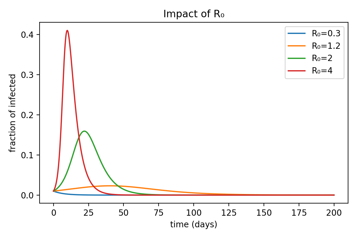
As expected, the number of infected individuals starts to decline immediately when $R_0 < 1$, while in the other cases it first rises to a peak before beginning to fall.

This phenomenon is due to saturation. As we mentioned earlier, the exponential solution holds only when the number of infected individuals is small — that is, when there are still plenty of susceptibles available to infect. As time passes, the spread becomes more difficult because the pool of susceptibles shrinks, replaced by infected or recovered individuals (who, in our model, cannot be infected again).

One might wonder: what role does the $\mu$ that appears in the exponential formula, next to $R_0$, actually play?
It is simply a time-scaling factor: diseases with the same $R_0$ but different $\mu$ values will spread in the same way, but over different time scales.

Notice in the figure that the maximum fraction of infected individuals reached is always the same — only shifted in time depending on the value of $\mu$.

The Danger of an Epidemic

Let’s now try to understand what these values actually mean.
Imagine a disease with $R_0 = 2$ — let’s be optimistic compared to the coronavirus — and look at how the number of infected individuals evolves over time.

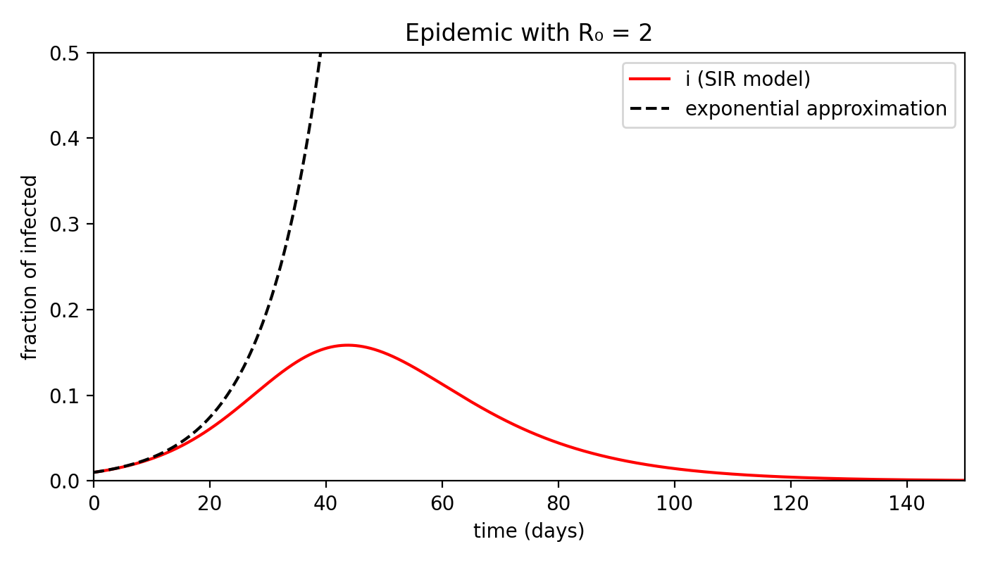
First of all, we can see that the exponential prediction quickly diverges from reality: assuming the time scale is measured in days, after about three weeks saturation has already begun.
The peak of infections occurs around day 40, after which the curve starts to decline. By day 150, there are no infected individuals left.

I should emphasize that these numbers are not meant to be precise — they serve only to illustrate the phenomenon qualitatively.
Don’t take them as predictions of a six-month quarantine (at least, not based on this model!).

If we look at the peak, however, it becomes clear why there is cause for concern: around day 40, almost 18% of the population is infected!
In a population of 60 million, that means nearly 11 million people.
This is an enormous — and alarming — number. But that’s not the end of the story.
Let’s also examine how $s$ and $r$ evolve over time, alongside the infected population.

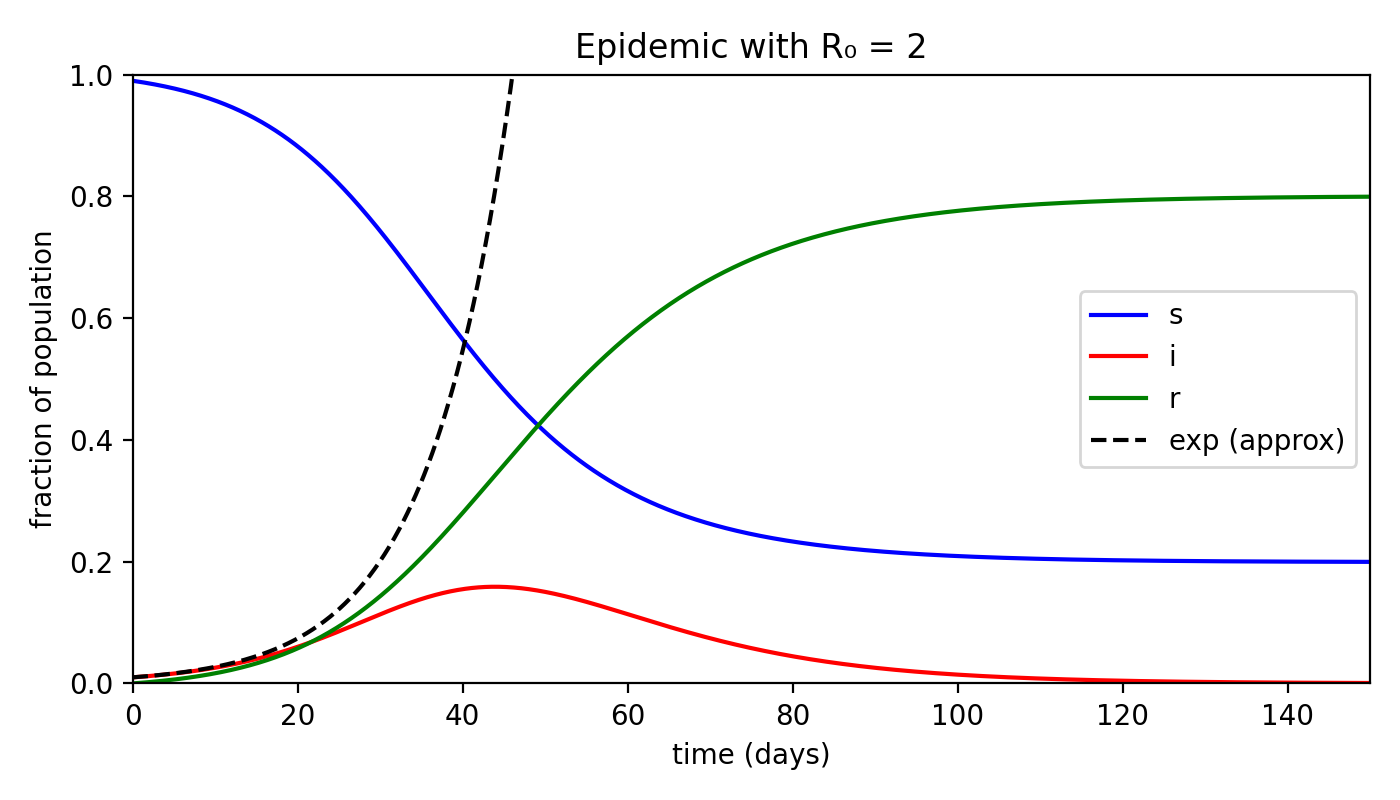
Incredible, isn’t it? By the end of the epidemic — that is, when $i = 0$ — almost 80% of the population has been infected and moved into the removed category!

Assuming a case fatality rate (the proportion of deaths among infected individuals, which in our model corresponds to $r$) of about 4% — roughly the estimated value for COVID-19 — the overall mortality (deaths as a fraction of the total population) would be 3.2%.
That would mean nearly two million deaths in a population of 60 million — a truly staggering number.
This is why such strict containment measures are being taken: the danger is immense.

So, what can be done?
As we have seen, $R_0$ depends on $\beta$ and $\mu$, which are properties of the pathogen and therefore difficult to change.
However, there is another parameter: $k$, the average number of contacts a person has per unit of time.
And this is precisely what restrictive measures target — by encouraging people to stay home and avoid crowded places, we reduce the number of contacts and thus lower $R_0$.

I am neither a doctor nor an epidemiologist. The purpose of this article is simply to show how even a basic mathematical model can explain a complex phenomenon like the spread of an epidemic, and to give meaning to the strict measures we have all experienced.

The sources of inspiration for this piece were the excellent 3Blue1Brown video and Chapter 10 of Barabási’s Network Science, which also discusses more sophisticated contagion models that take into account social networks and the effects of vaccination.

Stay well — and stay isolated.