When dealing with dynamical systems, one usually faces the problem of partially-observed data. The engineering literature deals a lot with partially-observed linear dynamical systems, but do we have any hope to make predictions when our system is nonlinear? To answer this question, we will have to discuss one of the most amazing results in this context: Takens’s theorem, which actually allows us to give a positive answer to this question.

In this post, I’ll quickly discuss this fundamental theorem and show how we can use it to predict dynamical systems, providing some coding examples in Python (using also scikit-learn and Pytorch) to guide you through it.

Stating the Problem

Let us consider a (possibly nonlinear) dynamical system, which we write of the form:

\begin{equation}\label{eqn:takens_source} s_{t} = g(s_{t-1}) \end{equation}

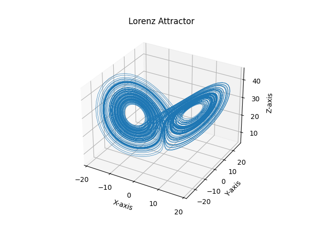
For example, we can use the Lorenz system as in the previous example.

# Define the Lorenz system of differential equations
def lorenz(t, y, sigma, rho, beta):
    dydt = [sigma * (y[1] - y[0]),
            y[0] * (rho - y[2]) - y[1],
            y[0] * y[1] - beta * y[2]]
    return dydt

# Set the parameters
sigma = 10.0
rho = 28.0
beta = 8.0 / 3.0

# Set the initial conditions
initial_conditions = [1.0, 0.0, 20.0]

# Set the time span for integration
t_span = (0, 100)
t_eval = np.linspace(t_span[0], t_span[1], 12000)

# Solve the system of differential equations
sol = solve_ivp(lorenz, t_span, initial_conditions, args=(sigma, rho, beta), t_eval=t_eval)

You may argue that the Lorenz System is continuous-time dynamical system, but as discussed here one can always construct a discrete-time dynamical system starting from that: in fact, everytime you measure a system, you’ll always deal with discrete observations in time. Let’s now plot one orbit and recognize the famous attractor.

Observables

Usually things get even more complicated when dealing with real systems. For example, in many applications it happens that we do not have access to the full state of the system, but only to an observation of its state.

\begin{equation}\label{eqn:takens_observable} u_{t}= h(s_{t}) \end{equation}

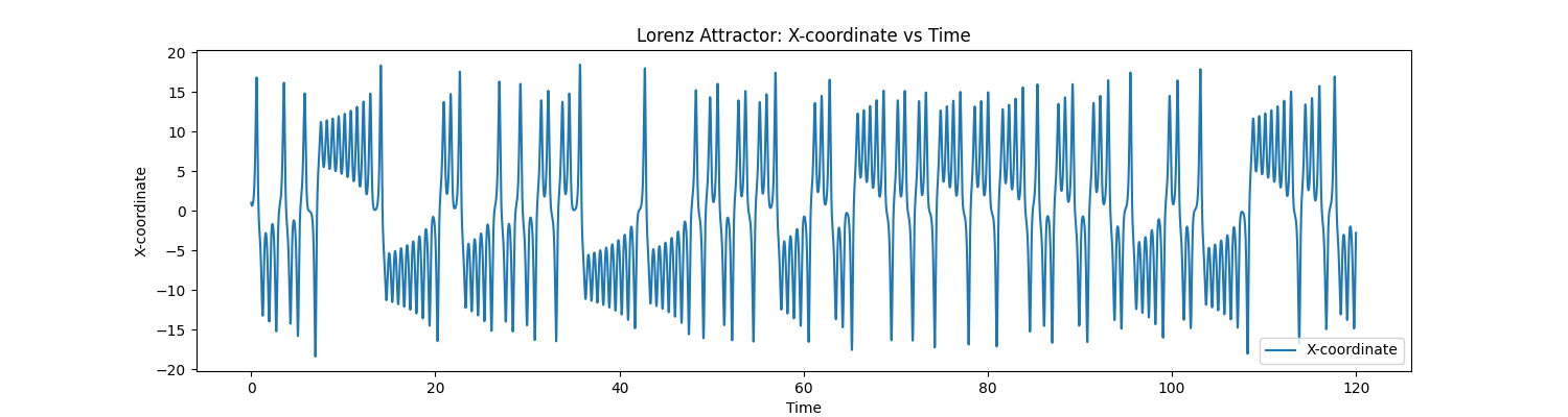
where we call $u_t$ the observable. Each orbit of \eqref{eqn:takens_source} {$s_t$} corresponds to a time realization of \eqref{eqn:takens_observable} {$u_t$}. In this post, we consider the symple case in which $u_t$ is simply one of the coordinates ($x$) of the Lorenz System.

    # Extract the x-coordinate (u)
    u = sol.y[0]
    
    #create train and test
    u_train = u[500:10000] # we discard some initial points
    u_test = u[10000:]

In this case, the data at our disposal looks like this:

TAKENS’S THEOREM

Since \eqref{eqn:takens_source} is an autonomous system, the initial condition $s_{t_{0}}$ determines the entire evolution of the system and, consequently, the entire realization of the observable. This means that the entire sequence {${u}_t$} depends on the initial condition, in the sense that different initial conditions will lead to different state sequences.

We now wonder whether the opposite is true or not, i.e., if one can reconstruct the state of the system by observing a series of one-dimensional measures like \eqref{eqn:takens_observable}.
Takens’s theorem deals with this question. In order to state the theorem, we now introduce a delay vector $x_t$ constructed from the observation of our dynamical system as:

where $F_D: \mathbb{R}^d \to \mathbb{R}^D$ is the $D$-delay map. Its smoothness depends on the smoothness of $g$ and $h$.

Let’s code this operation:

# Create a delay embedding
def delay_embedding(data, d, tau):
    N = len(data)
    indices = np.arange(d) * tau + np.arange(N - (d - 1) * tau)[:, None]
    embedded_data = data[indices]
    return embedded_data

For example:

arr = np.array([1,2,3,4,5,6,7,8,9])
emb = delay_embedding(arr,4,2)
emb

Will lead to this output

array([[1, 3, 5, 7],
       [2, 4, 6, 8],

We can apply this function to create the delay embedding of our data:

# Set parameters for delay embedding
d = 20  # Number of delays
tau = 1  # Time delay

# Create delay embedding
embedded_data = delay_embedding(u_train, d, tau)

If we assume that the motion of \eqref{eqn:takens_source} occurs in manifold $\mathcal{M}$ of dimension $d$, we call $\mathcal{H}_D \subset \mathbb{R}^D$ its image under the effect of $F_D$. So, we can now present a different formulation of the question above: is $F_D$ a diffeormorphism? The answer to this question in given by the Takens’s Embedding Theorem, which we now state (in a fairly informal version):

Takens’s Embedding Theorem [^1]

Let $\mathcal{M}$ be a compact $d$-dimensional $C^2$ manifold. For almost any pair of function $g$ and $h$, which are continuously differentiable on $\mathcal{M}$, the mapping

given by \eqref{eqn:takens_function} is a diffeomorphism any $D > 2d$.

This paper [^2] gives a really detailed description of the theorem, also discussing its implication in signal processing. Practically this can roughly be interpreted as stating that our delay embedding vector ${x}_t$ encode information about the full state $s_t$ even if we did not (and can not) observe it! To see this, let’s perform the singular value decomposition on our delay embedding:

# Perform Singular Value Decomposition (SVD) on the transposed embedded data
U, S, vh = np.linalg.svd(embedded_data.T)

# Plot the singular values
plt.plot(range(1, len(S) + 1), S, marker='o')
plt.xlabel('Singular Value Index')
plt.ylabel('Singular Value')
plt.title('Singular Value Decomposition')
plt.savefig("SVD")
plt.show()

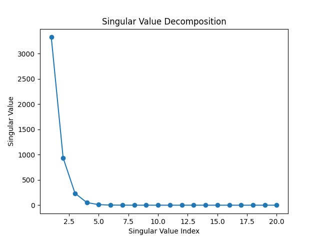
We see that the first 3 dimensions encode most of the information: let’s see what happens when we plot them.

# Plot the first three rows of vh
fig = plt.figure()
ax = fig.add_subplot(111, projection='3d')
ax.plot(vh[0], vh[1], vh[2], lw=0.5)
ax.set_xlabel('X-axis')
ax.set_ylabel('Y-axis')
ax.set_zlabel('Z-axis')
ax.set_title('Lorenz Attractor')
plt.savefig("Lorenz_reconstructed")
plt.show()

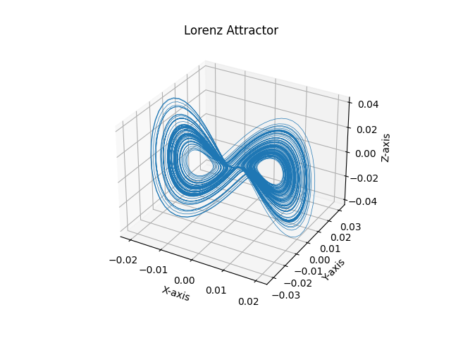
Well, this looks fairly similar to the original attractor! Notice that there is no way we can get exactly the attractor, as we never observed the real values of the second and third components ($y$ and $z$), but what we get is something that has the same topology (we have the two ‘‘wings’’ with holes in the middle).

Implication for Machine Learning

This implies that $\mathcal{H}_D$ is an embedding of $\mathcal{M}$ which, in turn, means that each vector $ {x}$ on $\mathcal{H}_D$ corresponds to a unique vector $ {s}$ on $\mathcal{M}$. So $ {x}_t$ can be used as a state vector to describe the dynamics of the original system \eqref{eqn:takens_source}. More specifically, an operator $ {\Gamma}$ might be introduced, such that:

\begin{equation}\label{eqn:takens_gamma} {x}_{t+1} = {\Gamma}( {x}_t) \end{equation}

where

\begin{equation}\label{eqn:takens_gamma_expanded} {\Gamma} := {F}_D \circ {g} \circ {F}_D^{-1} . \end{equation}

It is clear from \eqref{eqn:takens_function} that $x^i_{t+1} = \Gamma^i( {x}) = x^{i-1}= u_{t-i}$ for $i \le 2$. The only component which actually needs to be predicted is the first one, i.e.,

\begin{equation}\label{eqn:Psi} u_{t+1} = x^1{t+1} = \Gamma^1( {x}_t) := \Psi(u_t,u{t-1}, \dots, u_{t-(D-1)}). \end{equation}

Where $\Psi$ is a function that is able to produce the next element of our time series ($u_{t+1}$) by reading the past $D$ elements – i.e., the vector $ {x}_t$.

Linear Model

The function $\Psi$ is guaranteed to exist by Takens’s Theorem, in particular by Eq.~\ref{eqn:takens_gamma_expanded}, but we don’t know how it looks like. And what do we do in this kind of situation? We try to learn it!

As a first attempt we can go with a basic linear model.

from sklearn import linear_model

X = embedded_data[:-1,:]
Y = embedded_data[1:,-1]

linear_predictor = linear_model.Ridge(alpha = 1e-5)

linear_predictor.fit(X,Y)

So, linear_predictor is our (linear) approximation of $\Psi$. Let’s see how we did:

Well, it doesn’t look so bad! But as discussed previously, learning dynamical systems is not that simple: we must also make sure that our model is able to generate good trajectories when running autonomously. To do that we will iteratively apply Eq. \eqref{eqn:Psi}:

x_start=X[-1,:]
x_start = x_start[ np.newaxis,:]
L_seq = 900
x = x_start

preds = []
for _ in range(L_seq):
    pred = linear_predictor.predict(x)
    preds.append(pred)
    x = np.concatenate((x[:,1:],pred[np.newaxis,:]), axis=1)

Let’s see what we get.

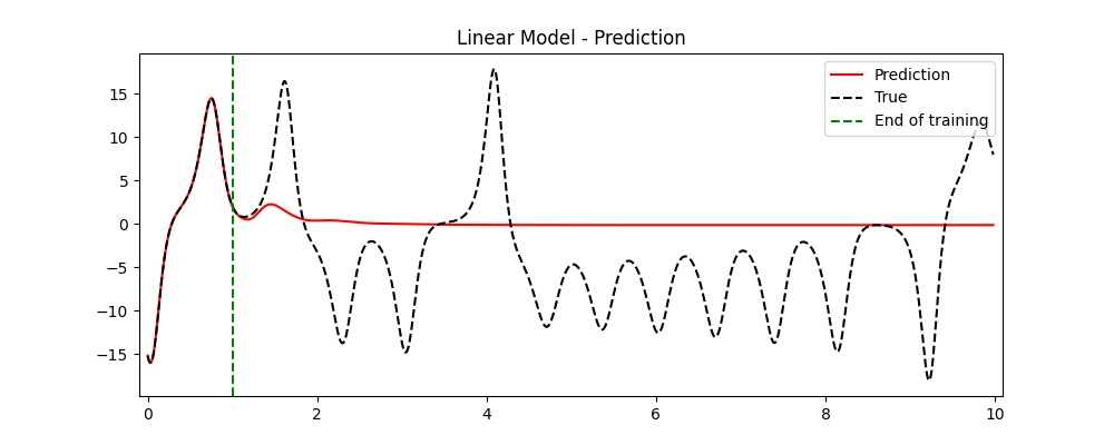
Unfortunately, after a short time our trajectory becomes a boring line, failing to represent all the complex dynamical features displayed by our system. But this was expected: dynamical linear models can only have simple behaviors. What can we do include some nonlinearities?

Neural Network

In fact, we can try to approximated $\Psi$ using a neural network. In Pytorch, this can be done in only a few lines of code.

import torch
import torch.nn as nn
import torch.optim as optim
from torch.utils.data import TensorDataset, DataLoader
import matplotlib.pyplot as plt

# Convert NumPy arrays to PyTorch tensors
X_tensor = torch.tensor(X, dtype=torch.float32)
Y_tensor = torch.tensor(Y, dtype=torch.float32)

# Create a simple neural network model
class NeuralNetwork(nn.Module):
    def __init__(self, input_dim, hidden_dim):
        super(NeuralNetwork, self).__init__()
        self.fc1 = nn.Linear(input_dim, hidden_dim)
        self.fc2 = nn.Linear(hidden_dim, hidden_dim)
        self.fc3 = nn.Linear(hidden_dim, 1)

    def forward(self, x):
        x = torch.relu(self.fc1(x))
        x = torch.relu(self.fc2(x))
        x = self.fc3(x)
        return x

# Set seeds for reproducibility
seed = 42
np.random.seed(seed)
torch.manual_seed(seed)


# Hyperparameters
input_dim = X.shape[1]
hidden_dim = 128
learning_rate = 1e-4
num_epochs = 100
batch_size = 32


# Create the neural network model
model = NeuralNetwork(input_dim, hidden_dim)

# Loss function and optimizer
criterion = nn.MSELoss()
optimizer = optim.Adam(model.parameters(), lr=learning_rate)

# Create a DataLoader for batching
dataset = TensorDataset(X_tensor, Y_tensor)
dataloader = DataLoader(dataset, batch_size=batch_size, shuffle=True)

# Lists to store loss history
loss_history = []

# Training loop
for epoch in range(num_epochs):
    for inputs, targets in dataloader:
        optimizer.zero_grad()
        outputs = model(inputs)
        loss = criterion(outputs, targets.view(-1, 1))
        loss.backward()
        optimizer.step()

    if epoch % 10 == 0:
        print(f"Epoch {epoch}, Loss: {loss.item()}")

    # Append the current loss to the loss history list
    loss_history.append(loss.item())

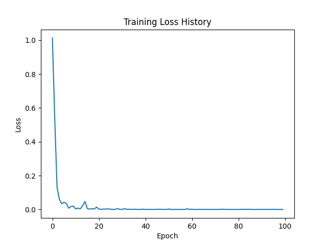
Well maybe 100 epochs were a bit of an overshooting, but let’s see how we performed.

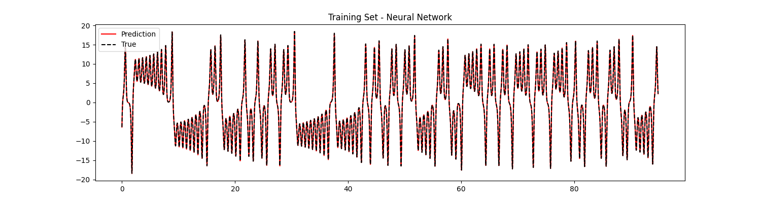
This looks perfect, but remember that also in the linear case we had perfect fitting for the train set. Let’s use our model to continue the trajectory.

x_start=X[-1,:]
x_start = x_start[ np.newaxis,:]
x_start=torch.tensor(x_start, dtype=torch.float32)
L_seq = 1500
x = x_start

nn_preds = []
for _ in range(L_seq):
    pred = model(x)
    nn_preds.append(pred.detach().numpy()[0])
    x = torch.concatenate((x[:,1:],pred), axis=1)

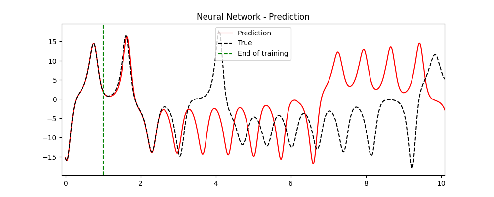
This looks really great! It is true that after some time the trajectories diverge, but the prediction of our model is not just a boring line, but something that really resembles a real trajectory of the Lorenz System! This fact, known as climate replication, is a good indication that our model has accurately learned the real dynamics of the system. Notice that since the original system is chaotic, there is no way of staying close to the real trajectory forever (as small errors will propagate).

Conclusions

Playing a bit with the parameters of the model and experimenting with the embedding, one can presumably do even better than that. All the code is available in this colab notebook. But the point of this post is that Takens’s theorem provides a really good theoretical tool to predict dynamical system, even when they are only partially observed! It is true that in real-world applications, it is impossible to check whether the conditions of Takens’s Theorem are fulfilled and the dimension $d$ is not known, so that it may appear that it has few practical implications. Yet, the theoretical value of this result is high.
In fact, Takens’s Theorem provides a formal justification for the autoregressive model which aim at predicting the future of time series from past observations.

[^1] Takens, Floris. “Detecting strange attractors in turbulence.” Lecture Notes in Mathematics, Berlin Springer Verlag 898 (1981): 366. [^2] Huke, J. P. “Embedding nonlinear dynamical systems: A guide to Takens’ theorem.” (2006).